Constant Likelihood
Managing plateaus in nested sampling is tricky because the measure of enclosed prior volume is assumed to be monotonically decreasing. In this simple model, the model is simply,
\(L(x) = P(y | x) = 1\)
and
\(P(x) = \mathcal{U}[x \mid 0, 1]\).
The analytic evidence for this model is,
\(Z = P(y) = \int_\mathcal{X} L(x) p(x) \,\mathrm{d} x = 1\)
[1]:
import tensorflow_probability.substrates.jax as tfp
from jax import random

tfpd = tfp.distributions
[2]:
from jaxns import Prior, Model


def log_likelihood(theta):
    return 0.


def prior_model():
    x = yield Prior(tfpd.Uniform(0., 1.), name='x')
    return x


model = Model(prior_model=prior_model,
              log_likelihood=log_likelihood)

log_Z_true = 0.
print(f"True log(Z)={log_Z_true}")
/home/albert/miniconda3/envs/jaxns_py/lib/python3.11/site-packages/jaxns/internals/mixed_precision.py:15: UserWarning: JAX x64 is not enabled. Setting it now. Check for errors.
  warnings.warn("JAX x64 is not enabled. Setting it now. Check for errors.")
INFO:jax._src.xla_bridge:Unable to initialize backend 'cuda':
INFO:jax._src.xla_bridge:Unable to initialize backend 'rocm': module 'jaxlib.xla_extension' has no attribute 'GpuAllocatorConfig'
INFO:jax._src.xla_bridge:Unable to initialize backend 'tpu': INTERNAL: Failed to open libtpu.so: libtpu.so: cannot open shared object file: No such file or directory
WARNING:jax._src.xla_bridge:An NVIDIA GPU may be present on this machine, but a CUDA-enabled jaxlib is not installed. Falling back to cpu.
True log(Z)=0.0
[3]:
from jaxns import NestedSampler

# Create the nested sampler class. In this case without any tuning.
exact_ns = NestedSampler(model=model, max_samples=1e4)

termination_reason, state = exact_ns(random.PRNGKey(42))
results = exact_ns.to_results(termination_reason=termination_reason, state=state)
/home/albert/miniconda3/envs/jaxns_py/lib/python3.11/site-packages/jaxns/internals/mixed_precision.py:61: UserWarning: Expected integer type, got bool, at public.py:173 in to_results -> sharded_static.py:475 in _to_results -> mixed_precision.py:105 in cast_to_count -> mixed_precision.py:67 in _cast_integer_to -> tree.py:61 in map -> tree_util.py:321 in tree_map -> tree_util.py:321 in <genexpr> -> mixed_precision.py:61 in conditional_cast.
  warnings.warn(f"Expected integer type, got {x.dtype}, {get_grandparent_info()}.")
[4]:
# We can use the summary utility to display results
exact_ns.summary(results)
--------
Termination Conditions:
All live-points are on a single plateau (potential numerical errors, consider 64-bit)
--------
likelihood evals: 30
samples: 45
phantom samples: 0
likelihood evals / sample: 0.7
phantom fraction (%): 0.0%
--------
logZ=-0.034 +- 0.023
max(logL)=0.0
H=-0.03
ESS=20
--------
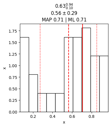
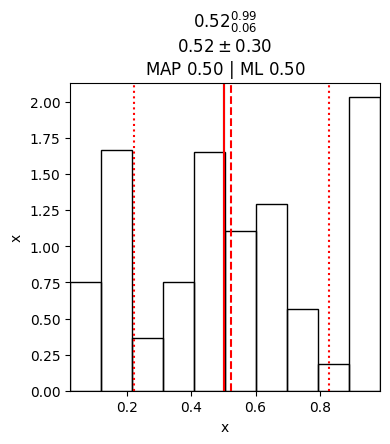
x: mean +- std.dev. | 10%ile / 50%ile / 90%ile | MAP est. | max(L) est.
x: 0.51 +- 0.3 | 0.13 / 0.47 / 0.96 | 0.5 | 0.5
--------
[5]:
# We plot useful diagnostics and a distribution cornerplot
exact_ns.plot_diagnostics(results)
exact_ns.plot_cornerplot(results)
/home/albert/miniconda3/envs/jaxns_py/lib/python3.11/site-packages/jaxns/plotting.py:48: UserWarning: Found samples with zero likelihood evaluations.
  warnings.warn("Found samples with zero likelihood evaluations.")
/home/albert/miniconda3/envs/jaxns_py/lib/python3.11/site-packages/jaxns/plotting.py:52: RuntimeWarning: divide by zero encountered in divide
  1. / num_likelihood_evaluations_per_sample