Lennard-Jones Potentials for modelling phase transitions in materials
Nested Sampling is the ideal tool for computing the partition function.
where \(\beta \in [0, \infty)\) is the inverse temperature parameter \(\beta=(k_B T)^{-1}\), \(\mathcal{X}\) is the set of all configurations of the system, and \(E : \mathcal{X} \to \mathbb{R}\) is the potential function, which in this case will be the Lennard-Jones potential,
In this equation, the \(-\epsilon\) represents the energy of the ground state, and \(\sigma\) is the equilibrium distance when the potential energy is zero.
The system is invariant to changes in sigma and the total size of the region. Therefore, we choose \(\sigma\) as a ratio with the size of the box. We’ll chose to sample states within a unit box, therefore, we are choosing how big the box is in units of \(\sigma\). Choosing \(\sigma=0.01\) is equivalent to choosing, means the volume is roughly 100 particles per side.
[21]:
import jax

jax.config.update("jax_enable_x64", True)

import tensorflow_probability.substrates.jax as tfp
from jax import random, numpy as jnp
from jax import vmap

from jaxns import Model
from jaxns import Prior

tfpd = tfp.distributions
[22]:
def pairwise_distances_squared(points):
    n = points.shape[0]
    pair_indices = jnp.triu_indices(n, 1)  # Upper triangular indices, excluding diagonal

    # Create function that calculates the distance between two points
    def dist_fn(ij):
        i, j = ij
        return jnp.sum(jnp.square(points[i] - points[j]))

    # Apply this function to each pair of indices
    pairwise_distances = vmap(dist_fn)(pair_indices)

    return pairwise_distances


# test pairwise_distances_squared
points = jnp.array([[1, 2], [3, 4], [5, 6], [7, 8]])
assert jnp.all(pairwise_distances_squared(points) == jnp.asarray([8, 32, 72, 8, 32, 8]))
[23]:
from jaxns.internals.log_semiring import LogSpace
import jaxns.framework.context as ctx

num_particles = 7
num_pairs = num_particles * (num_particles - 1) // 2
sigma = jnp.asarray(1., jnp.float64) # 0.3405 nm
box_size = jnp.asarray(1.56, jnp.float64)  # 4 sigma in each direction
epsilon_over_beta = jnp.asarray(119.8, jnp.float64)  # 119.8 K
k_B = jnp.asarray(1.38064852e-23, jnp.float64)  # J/K
beta_init = epsilon_over_beta / 300. # Simulate at 300 K


def prior_model():
    x = yield Prior(
        tfpd.Uniform(
            low=jnp.zeros((num_particles, 3)),
            high=box_size * jnp.ones((num_particles, 3))),
        name='x'
    )
    beta = ctx.get_parameter('beta', init=beta_init, dtype=jnp.float64)
    return x, beta


def log_likelihood(x, beta):
    """
    negative V12-6 potential.
    """
    r2_ij = pairwise_distances_squared(x / sigma)
    r6_ij = r2_ij ** 3
    r12_ij = r6_ij ** 2
    r6_ij_inv = jnp.reciprocal(r6_ij)
    r12_ij_inv = jnp.reciprocal(r12_ij)
    E_pairs = 4. * (r12_ij_inv - r6_ij_inv)
    E = jnp.sum(E_pairs)
    return -beta * E


model = Model(
    prior_model=prior_model,
    log_likelihood=log_likelihood
)
params = model.params

print(params)

model.sanity_check(random.PRNGKey(42), 1000)
/home/albert/git/jaxns/jaxns/framework/context.py:98: UserWarning: Using a constant initializer for state. This is not recommended as it may induce closure issues.
  warnings.warn(
{'beta': Array(0.39933333, dtype=float64)}
INFO:jaxns:Sanity check...
INFO:jaxns:Sanity check passed
[24]:
import jax
from jaxns import NestedSampler, TerminationCondition
# Create the nested sampler class. In this case without any tuning.
ns = NestedSampler(
model=model,
max_samples=500000,
shell_fraction=0.
)
# Crucial for Lenard-Jones potential is to go deep enough.
# Since we know min(E)=-1 for a single pair, we know that the log_L_max = num_pairs
# Thus we can use the log_L_contour termination condition.
term_cond = TerminationCondition(
log_L_contour=0.9995 * num_pairs
)
ns_compiled = jax.jit(ns).lower(jax.random.PRNGKey(42), term_cond=term_cond).compile()
termination_reason, state = ns_compiled(random.PRNGKey(42), term_cond=term_cond)
results = ns.to_results(
termination_reason=termination_reason,
state=state
)
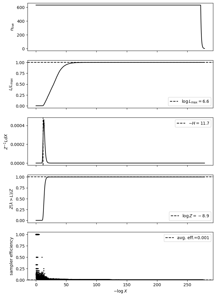
ns.summary(results)
ns.plot_diagnostics(results)
ns.save_results(results, 'results.json')
--------
Termination Conditions:
All live-points are on a single plateau (sign of possible precision error)
no seed points left (consider decreasing shell_fraction)
--------
likelihood evals: 189471362
samples: 172498
phantom samples: 0
likelihood evals / sample: 1098.4
phantom fraction (%): 0.0%
--------
logZ=-8.87 +- 0.14
max(logL)=6.59
H=-11.75
ESS=1598
--------
x[#]: mean +- std.dev. | 10%ile / 50%ile / 90%ile | MAP est. | max(L) est.
x[0]: 0.75 +- 0.55 | 0.08 / 0.6 / 1.49 | 0.0 | 0.0
x[1]: 0.82 +- 0.56 | 0.07 / 1.0 / 1.49 | 1.38 | 1.38
x[2]: 0.79 +- 0.56 | 0.08 / 0.89 / 1.49 | 0.62 | 0.62
x[3]: 0.88 +- 0.54 | 0.1 / 1.09 / 1.5 | 1.1 | 1.1
x[4]: 0.86 +- 0.55 | 0.09 / 1.04 / 1.5 | 1.17 | 1.17
x[5]: 0.7 +- 0.56 | 0.05 / 0.5 / 1.47 | 0.54 | 0.54
x[6]: 0.77 +- 0.54 | 0.09 / 0.73 / 1.48 | 1.27 | 1.27
x[7]: 0.73 +- 0.57 | 0.05 / 0.57 / 1.48 | 0.07 | 0.07
x[8]: 0.8 +- 0.55 | 0.08 / 0.86 / 1.5 | 0.56 | 0.56
x[9]: 0.63 +- 0.55 | 0.05 / 0.38 / 1.47 | 0.41 | 0.41
x[10]: 0.83 +- 0.54 | 0.09 / 0.97 / 1.49 | 0.48 | 0.48
x[11]: 0.78 +- 0.56 | 0.07 / 0.7 / 1.48 | 1.14 | 1.14
x[12]: 0.82 +- 0.55 | 0.08 / 0.95 / 1.49 | 0.67 | 0.67
x[13]: 0.87 +- 0.55 | 0.1 / 1.08 / 1.5 | 1.49 | 1.49
x[14]: 0.84 +- 0.56 | 0.08 / 1.0 / 1.51 | 1.52 | 1.52
x[15]: 0.72 +- 0.55 | 0.06 / 0.53 / 1.48 | 0.37 | 0.37
x[16]: 0.66 +- 0.53 | 0.06 / 0.47 / 1.46 | 0.5 | 0.5
x[17]: 0.8 +- 0.55 | 0.08 / 0.87 / 1.48 | 0.03 | 0.03
x[18]: 0.88 +- 0.55 | 0.09 / 1.1 / 1.5 | 1.45 | 1.45
x[19]: 0.68 +- 0.53 | 0.06 / 0.5 / 1.43 | 0.69 | 0.69
x[20]: 0.7 +- 0.54 | 0.07 / 0.58 / 1.46 | 1.48 | 1.48
--------
/home/albert/git/jaxns/jaxns/plotting.py:45: UserWarning: Found samples with zero likelihood evaluations.
  warnings.warn("Found samples with zero likelihood evaluations.")
[25]:
from typing import NamedTuple
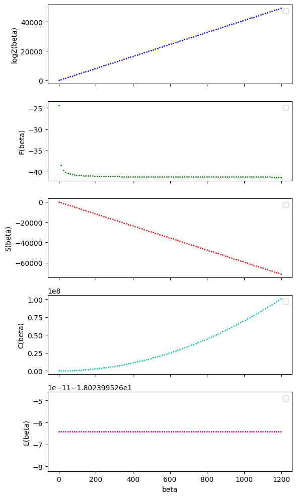
quantity_names = ['logZ(beta)', 'F(beta)', 'S(beta)', 'C(beta)', 'E(beta)']
colors = ['b', 'g', 'r', 'c', 'm']
class Quantities(NamedTuple):
logZ: jax.Array
F: jax.Array
S: jax.Array
C: jax.Array
E: jax.Array
class IntermediateQuantities(NamedTuple):
beta_E: jax.Array
beta_E2: jax.Array
def compute_integrands_of_interest(model, U) -> IntermediateQuantities:
# Divide out beta_init
beta_E = -model.forward(U) / beta_init # beta * E(x)
beta_E2 = beta_E ** 2
return IntermediateQuantities(beta_E=beta_E, beta_E2=beta_E2)
@jax.jit
def compute_quantities(beta) -> Quantities:
integrands = jax.vmap(
lambda U: compute_integrands_of_interest(model({'beta': beta}), U)
)(results.U_samples)
weights = LogSpace(results.log_dp_mean)
# Z(beta) = int exp(-beta E(x)) dx
Z_beta = (LogSpace(-integrands.beta_E) * weights).sum()
F_beta = -Z_beta.log_abs_val / beta
exp_beta_E = (LogSpace.from_signed_value(integrands.beta_E) * weights).sum()
exp_beta_E2 = (LogSpace.from_signed_value(integrands.beta_E2) * weights).sum()
S_beta = (exp_beta_E - Z_beta.log()).value
C_beta = (exp_beta_E2 - exp_beta_E ** 2).value
E_beta = (exp_beta_E / LogSpace(jnp.log(beta))).value
return Quantities(
logZ=Z_beta.log_abs_val,
F=F_beta,
S=S_beta,
C=C_beta,
E=E_beta
)
x = []
y = []
import pylab as plt
fig, axs = plt.subplots(len(quantity_names), 1, figsize=(6, len(quantity_names) * 2), squeeze=False, sharex=True)
T_min = 0.1 # K
T_max = 300 # K
beta_min = epsilon_over_beta / T_max
beta_max = epsilon_over_beta / T_min
for beta in jnp.linspace(beta_min, beta_max, 100):
quantities = compute_quantities(beta)
x.append(beta)
y.append(quantities)
for i, (name, q, c) in enumerate(zip(quantity_names, quantities, colors)):
axs[i, 0].scatter(beta, q, color=c, s=1)
for i, (name, c) in enumerate(zip(quantity_names, colors)):
axs[i, 0].set_ylabel(name)
# Only 1 label on legend, despite labelling each beta
axs[i, 0].legend()
axs[-1, 0].set_xlabel('beta')
plt.tight_layout()
plt.show()
2024-10-09 18:44:53.773979: E external/xla/xla/service/slow_operation_alarm.cc:65] Constant folding an instruction is taking > 2s:

  %negate = f64[172498,7,3]{2,1,0} negate(f64[172498,7,3]{2,1,0} %constant.37)

This isn't necessarily a bug; constant-folding is inherently a trade-off between compilation time and speed at runtime. XLA has some guards that attempt to keep constant folding from taking too long, but fundamentally you'll always be able to come up with an input program that takes a long time.

If you'd like to file a bug, run with envvar XLA_FLAGS=--xla_dump_to=/tmp/foo and attach the results.
2024-10-09 18:44:54.102546: E external/xla/xla/service/slow_operation_alarm.cc:133] The operation took 2.328634594s
Constant folding an instruction is taking > 2s:

  %negate = f64[172498,7,3]{2,1,0} negate(f64[172498,7,3]{2,1,0} %constant.37)

This isn't necessarily a bug; constant-folding is inherently a trade-off between compilation time and speed at runtime. XLA has some guards that attempt to keep constant folding from taking too long, but fundamentally you'll always be able to come up with an input program that takes a long time.

If you'd like to file a bug, run with envvar XLA_FLAGS=--xla_dump_to=/tmp/foo and attach the results.
WARNING:matplotlib.legend:No artists with labels found to put in legend.  Note that artists whose label start with an underscore are ignored when legend() is called with no argument.
WARNING:matplotlib.legend:No artists with labels found to put in legend.  Note that artists whose label start with an underscore are ignored when legend() is called with no argument.
WARNING:matplotlib.legend:No artists with labels found to put in legend.  Note that artists whose label start with an underscore are ignored when legend() is called with no argument.
WARNING:matplotlib.legend:No artists with labels found to put in legend.  Note that artists whose label start with an underscore are ignored when legend() is called with no argument.
WARNING:matplotlib.legend:No artists with labels found to put in legend.  Note that artists whose label start with an underscore are ignored when legend() is called with no argument.